Sampler

The Sampler can be used to simulate the process of running jobs with an interferometer-based photonic system, in which the same input is placed into the system many times and the output distribution measured. As this output from the system is inherently probabilistic, the output distribution will tend towards the true distribution as more samples are collected. The number of samples collected from the system will depend on resource constraints, but will never be infinite, meaning there will always be some small variation from the ideal distribution.

As sampling is predominately how a hardware system is utilised, it is very useful to be able to understand how the process will look like for a given job. To demonstrate sampling we will show how the 2 qubit CNOT gate from [RLBW02] can be tested with the emulator. The circuit to define this gate is shown below, it occupies 6 modes, where the 4 central modes c0, c1, t0 & t1 are used for qubit encoding.

import numpy as np

cnot_circuit = lw.PhotonicCircuit(6)

theta = np.arccos(1/3)
to_add = [
    (3, np.pi/2, 0), (0, theta, 0), (2, theta, np.pi), (4, theta, 0), (3, np.pi/2, 0)
]

for m, t, p in to_add:
    cnot_circuit.bs(m, reflectivity = 0.5)
    cnot_circuit.ps(m+1, t)
    cnot_circuit.bs(m, reflectivity = 0.5)
    cnot_circuit.ps(m+1, p)

Note that this CNOT gate requires a set of post-selection criteria to function correctly, but this will be discussed more later. We can view the created CNOT gate with display. Mode labels can be specified to mark the ancillary (a) control qubit (c) and target qubit (t) modes.

cnot_circuit.display(mode_labels = ["a0", "c0", "c1", "t0", "t1", "a1"])

An input state to the system also needs to be defined. In this case, we’ll choose the qubit state \(\ket{10}\), which should produce the state \(\ket{11}\) after the CNOT. Using the circuit above, it can be seen that \(\ket{10}\) translates to an input photon on mode c1 and t0, so the input state should be:

input_state = lw.State([0, 0, 1, 1, 0, 0])

Sampling

Once the circuit and input state are defined, these can then be used in the creation of the Sampler object. The target number of samples and a random seed is also configured.

sampler = lw.Sampler(cnot_circuit, input_state, 10000, random_seed = 1)

Once created, the sampling procedure can be run on a selected backend. The sampler currently supports both permanent and slos backends.

backend = emulator.Backend("slos")
results = backend.run(sampler)

This returns a SamplingResult object, which has a range of useful functionality, but primarily the plot method can be used to view the output counts from the sampling experiment.

results.plot()

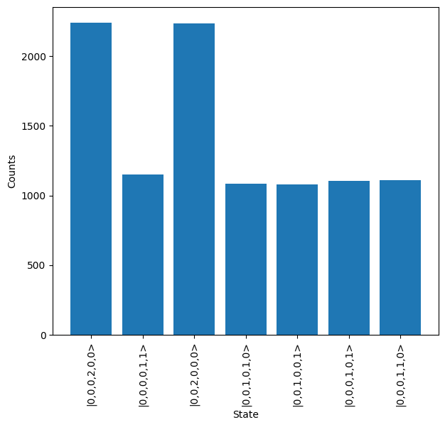
For the plot above, it can be seen there is no clear output, which is expected as the post-selection rules have not yet been applied. This is implemented in the next section.

Post-selection & Heralding

As mentioned, post-selection/heralding is required for the CNOT gate above to work correctly. In particular, the gate requires that no photons are measured on the a0 & a1 modes. Additionally, there is a condition that only one photon is measured across c0 & c1 and another across t0 & t1. These can be implemented by providing a function to the post_selection option on creation of the sampler or by assigning to the corresponding attribute. This can either be a dedicated function or can use the lambda function included with Python, but must take a single argument as the input, with this argument expected to be a State object. Alternatively, the built-in PostSelection object in the SDK can be used. There is also a min_detection option, which is used to set the minimum number of photons that should be detected at the output. In this case the function we supply will enforce this condition and so it is not necessary.

# Define post-selection function
def post_select(s):
    return not s[0] and not s[5] and sum(s[1:3]) == 1 and sum(s[3:5]) == 1

# Alternatively define as equivalent lambda function
post_select = lambda s: not s[0] and not s[5] and sum(s[1:3]) == 1 and sum(s[3:5]) == 1

# Or with post-selection object
post_select = lw.PostSelection()
post_select.add((1, 2), 1)
post_select.add((3, 4), 1)

sampler.post_selection = post_select
sampler.min_detection = 2 # Not required
sampler.sampling_mode = "input"

# Sample from the system again
results = backend.run(sampler)

# View results
results.plot()

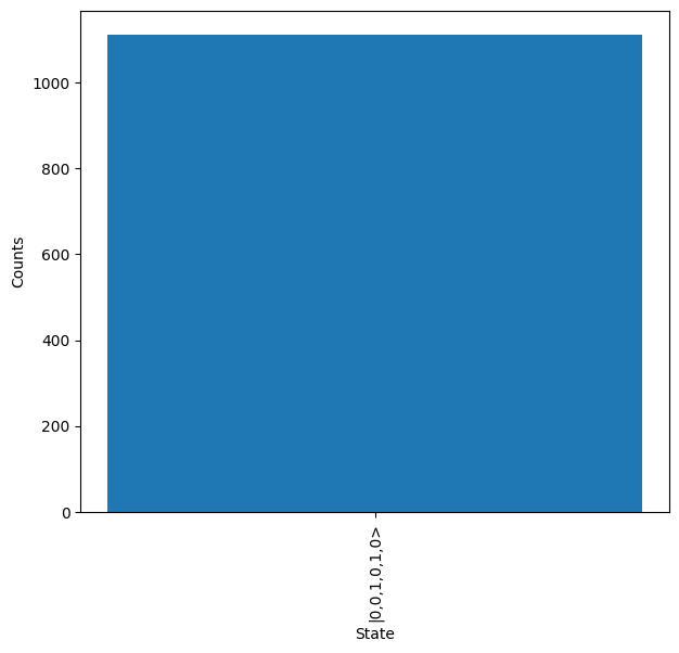
It can be seen from the output that the correct state is now measured, as \(\ket{001010}\) is equivalent to \(\ket{11}\) in qubit language. One important thing to notice is that the number of measured outputs is significantly less than the 10,000 inputs. This results from the 1/9 success probability of the gate, and the fact that the input sampling mode was used here, as this will generate 10,000 inputs to the system - some of which are then subsequently filtered out.